EDA notebook

This notebook contains the simple examples of EDA (exploratory data analysis) using ETNA library.

Table of Contents

• Creating TSDataset

• Visualization

  • Plot

  • Autocorrelation

  • Cross-correlation

  • Correlation heatmap

  • Distribution

• Outliers

  • Median method

  • Density method

import warnings
warnings.filterwarnings("ignore")

1. Creating TSDataset

Let’s load and look at the dataset

import pandas as pd

classic_df = pd.read_csv("data/example_dataset.csv")
classic_df.head()

	timestamp	segment	target
0	2019-01-01	segment_a	170
1	2019-01-02	segment_a	243
2	2019-01-03	segment_a	267
3	2019-01-04	segment_a	287
4	2019-01-05	segment_a	279

Our library works with the spacial data structure TSDataset. So, before starting the EDA, we need to convert the classical DataFrame to TSDataset.

from etna.datasets.tsdataset import TSDataset

To do this, we initially need to convert the classical DataFrame to the special format

df = TSDataset.to_dataset(classic_df)
df.head()

segment	segment_a	segment_b	segment_c	segment_d
feature	target	target	target	target
timestamp
2019-01-01	170	102	92	238
2019-01-02	243	123	107	358
2019-01-03	267	130	103	366
2019-01-04	287	138	103	385
2019-01-05	279	137	104	384

Now we can construct the TSDataset

ts = TSDataset(df, freq="D")
ts.head(5)

segment	segment_a	segment_b	segment_c	segment_d
feature	target	target	target	target
timestamp
2019-01-01	170	102	92	238
2019-01-02	243	123	107	358
2019-01-03	267	130	103	366
2019-01-04	287	138	103	385
2019-01-05	279	137	104	384

TSDataset has its own implementations of describe and info methods that gives information about distinct time series.

ts.describe()

	start_timestamp	end_timestamp	length	num_missing	num_segments	num_exogs	num_regressors	num_known_future	freq
segments
segment_a	2019-01-01	2019-11-30	334	0	4	0	0	0	D
segment_b	2019-01-01	2019-11-30	334	0	4	0	0	0	D
segment_c	2019-01-01	2019-11-30	334	0	4	0	0	0	D
segment_d	2019-01-01	2019-11-30	334	0	4	0	0	0	D

ts.info()

<class 'etna.datasets.TSDataset'>
num_segments: 4
num_exogs: 0
num_regressors: 0
num_known_future: 0
freq: D
          start_timestamp end_timestamp  length  num_missing
segments
segment_a      2019-01-01    2019-11-30     334            0
segment_b      2019-01-01    2019-11-30     334            0
segment_c      2019-01-01    2019-11-30     334            0
segment_d      2019-01-01    2019-11-30     334            0

2. Visualization

Our library provides a list of utilities for visual data exploration. So, having the dataset converted to TSDataset, now we can visualize it.

from etna.analysis import (
    cross_corr_plot,
    distribution_plot,
    sample_acf_plot,
    sample_pacf_plot,
    plot_correlation_matrix
)

2.1 Plotting time series

Let’s take a look at the time series in the dataset

ts.plot()

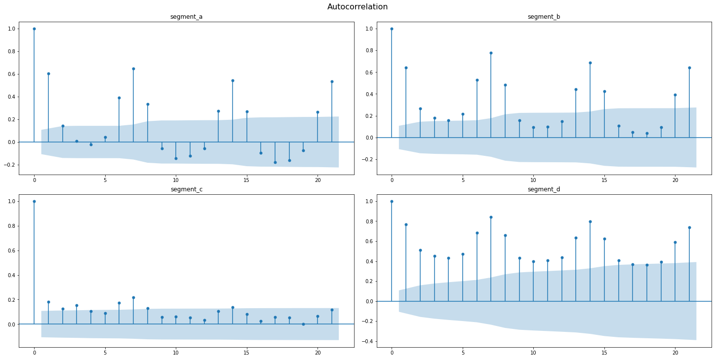
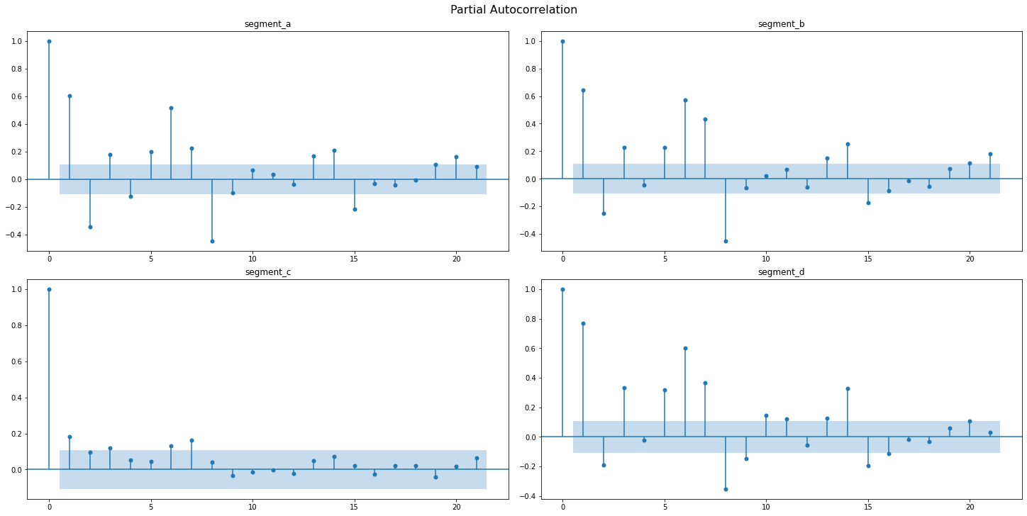
2.2 Autocorrelation & partial autocorrelation

Autocorrelation function(AFC) describes the direct relationship between an observation and its lag. The AFC plot can help to identify the extent of the lag in moving average models.

Partial autocorrelation function(PAFC) describes the direct relationship between an observation and its lag. The PAFC plot can help to identify the extent of the lag in autoregressive models.

Let’s observe the AFC and PAFC plot for our time series, specifying the maximum number of lags

sample_acf_plot(ts, lags=21)

sample_pacf_plot(ts, lags=21)

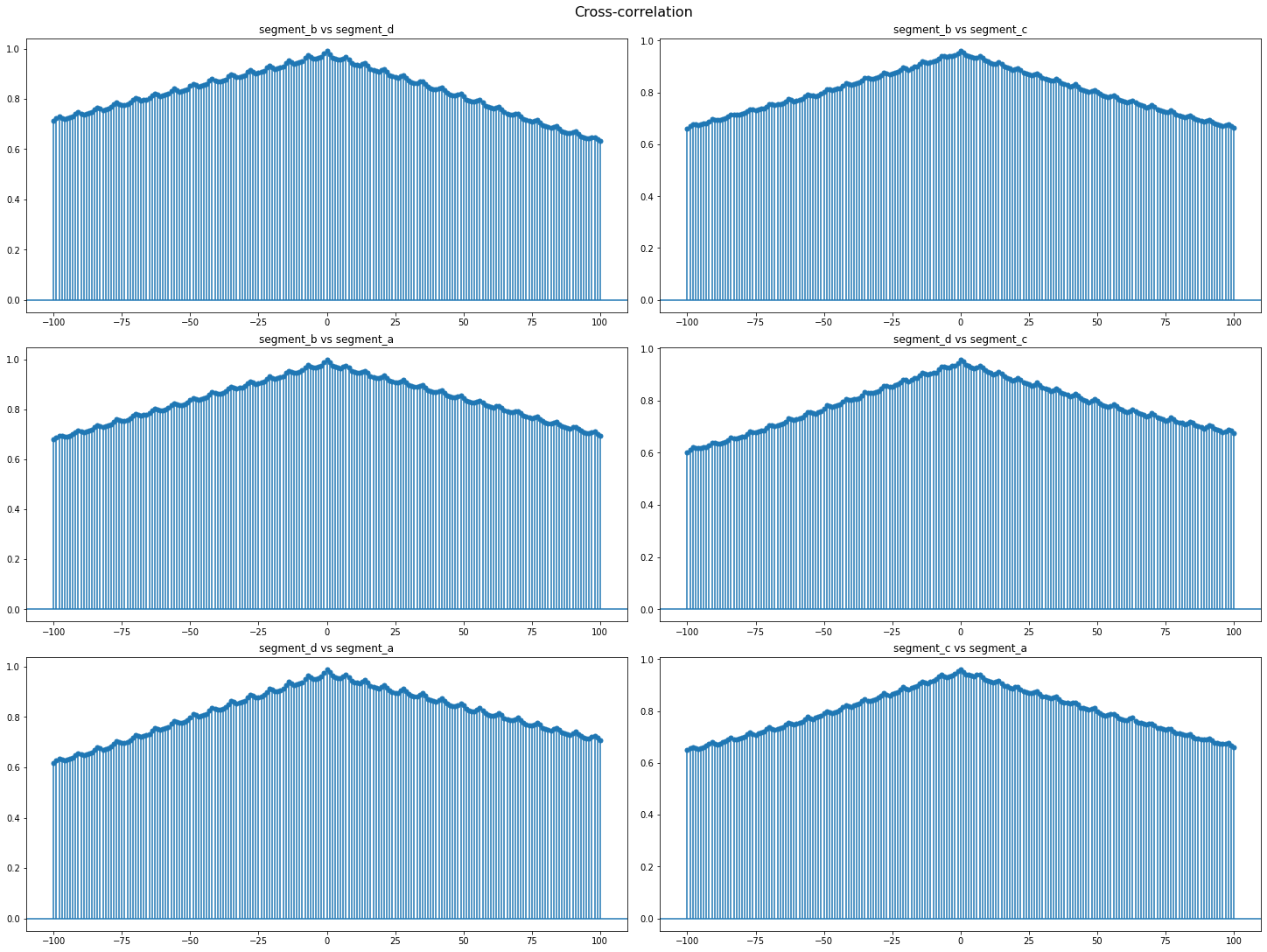
2.3 Cross-correlation

Cross-correlation is generally used to compare multiple time series and determine how well they match up with each other and, in particular, at what point the best match occurs. The closer the cross-correlation value is to \(1\), the more closely the sets are identical.

Let’s plot the cross-correlation for all pairs of time series in our dataset

cross_corr_plot(ts, maxlags=100)

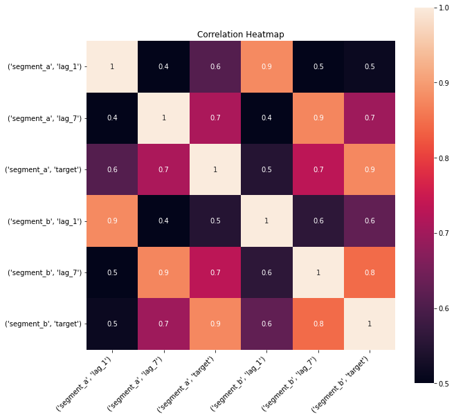
2.4 Correlation heatmap

Correlation heatmap is a visualization of pairwise correlation matrix between timeseries in a dataset. It is a simple visual tool which you may use to determine the correlated timeseries in your dataset.

Let’s take a look at the correlation heatmap, adding lags columns to the dataset to catch the series that are correlated but with some shift.

from etna.transforms import LagTransform

lags = LagTransform(in_column="target", lags=[1,7], out_column="lag")
ts.fit_transform([lags])

plot_correlation_matrix(ts, segments=["segment_a","segment_b"], method="spearman", vmin=0.5, vmax=1)

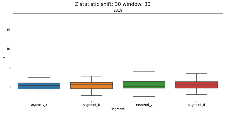
2.5 Distribution

Distribution of z-values grouped by segments and time frequency. Using this plot, you can monitor the data drifts over time.

Let’s compare the distributions over each year in the dataset

distribution_plot(ts, freq="1Y")

3. Outliers

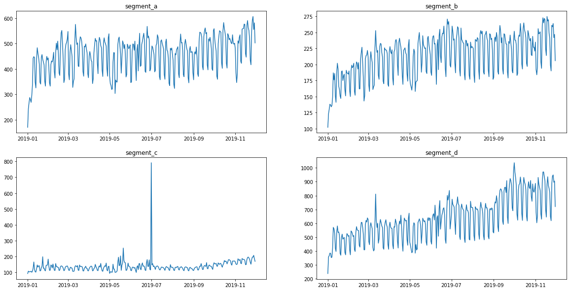
Visually, all the time series contain outliers - abnormal spikes on the plot. Their presence might cause the reduce in predictions quality.

ts.plot()

In our library, we provide two methods for outliers detection. In addition, you can easily visualize the detected outliers using plot_anomalies

from etna.analysis.outliers import get_anomalies_median, get_anomalies_density
from etna.analysis import plot_anomalies

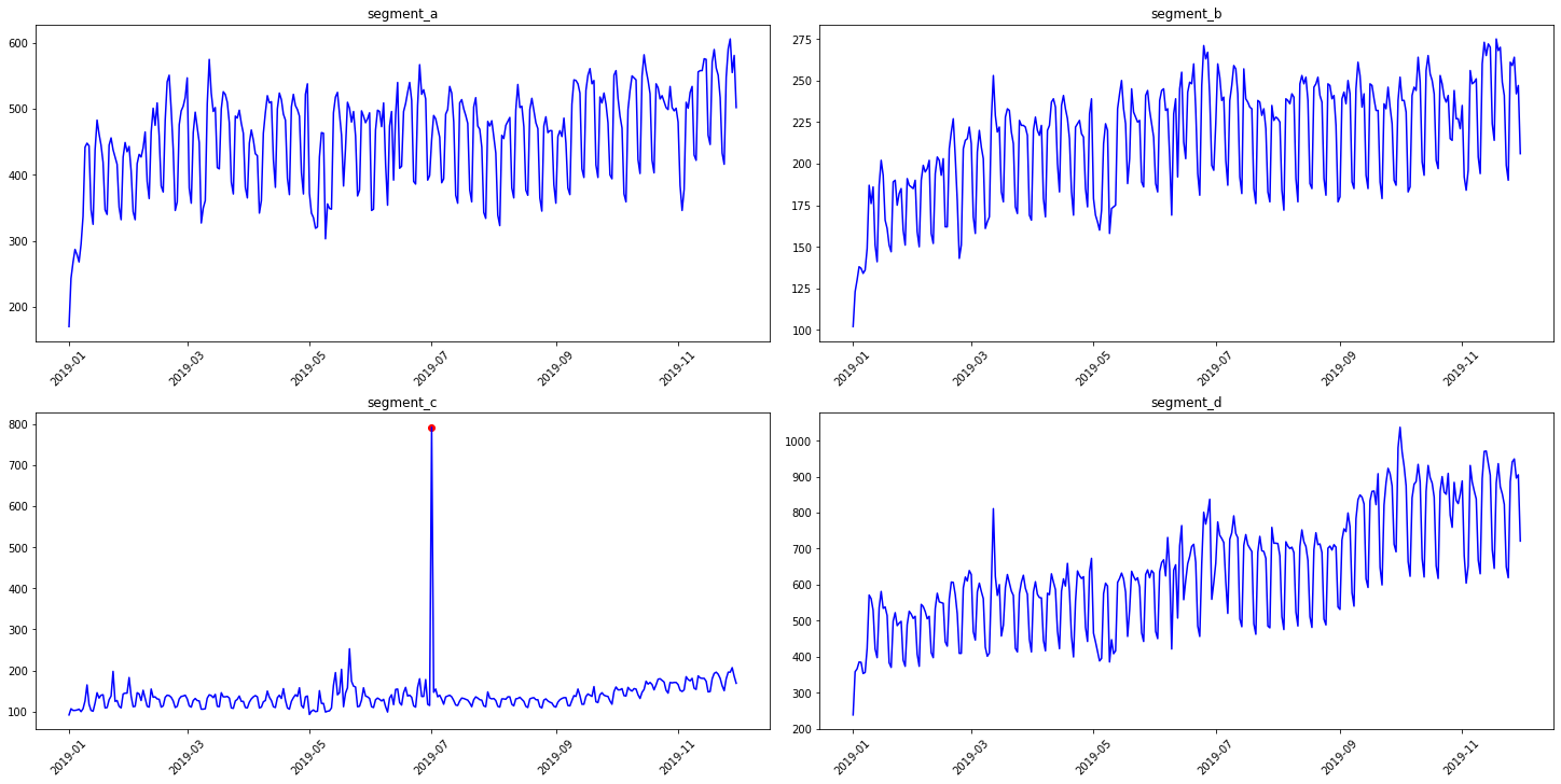
3.1 Median method

To obtain the point outliers using the median method we need to specify the window for fitting the median model.

anomaly_dict = get_anomalies_median(ts, window_size=100)
plot_anomalies(ts, anomaly_dict)

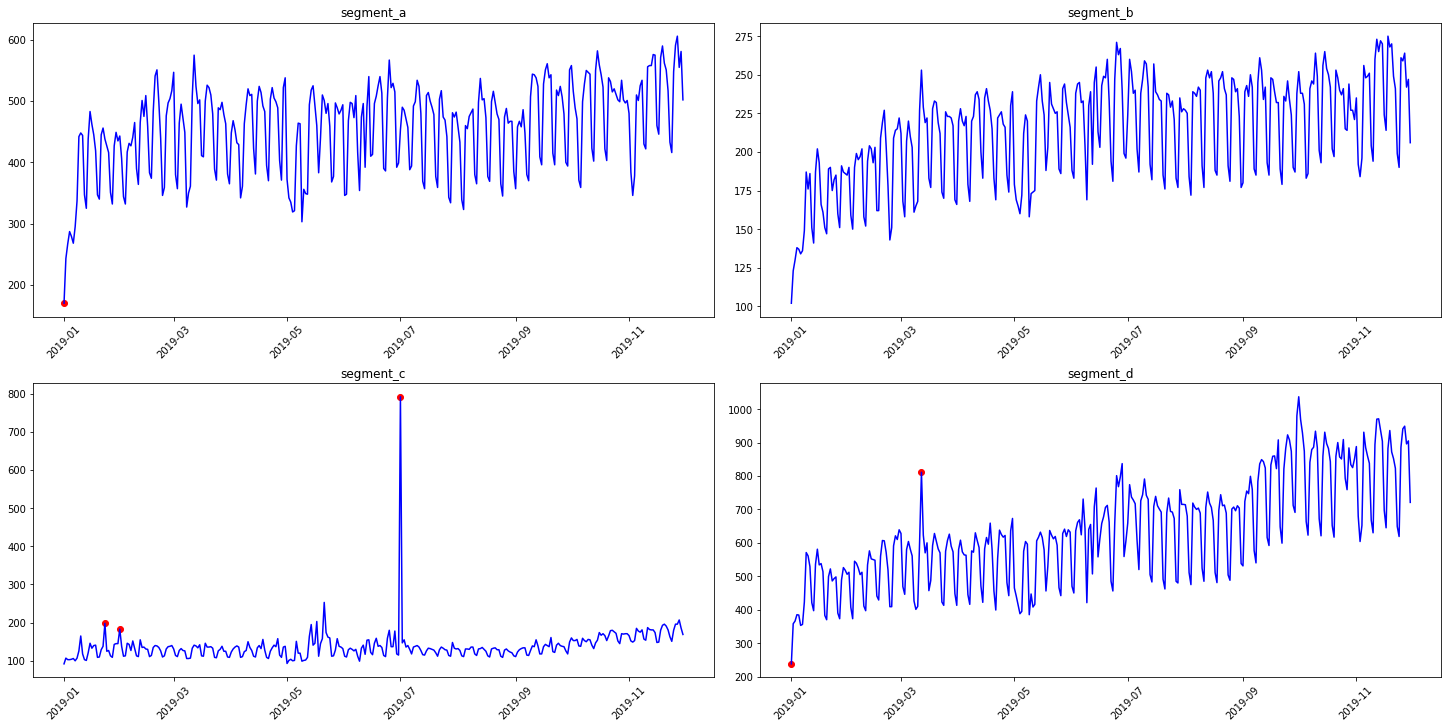
3.2 Density method

It is a distance-based method for outliers detection. Don’t rely on default parameters)

anomaly_dict = get_anomalies_density(ts)
plot_anomalies(ts, anomaly_dict)

The best practice here is to specify the method parameters for your data

anomaly_dict = get_anomalies_density(ts, window_size=18, distance_coef=1, n_neighbors=4)
plot_anomalies(ts, anomaly_dict)

That’s all for this notebook. More features for time series analysis you can find in our documentation.